Disclaimer: This article has nothing to do with corrections to the element Potassium, which is denoted as K in the periodic table.
Instead, it is about the corrections involved in astronomy, especially photometric and/or spectrometric calibrations between objects observed at different redshifts.
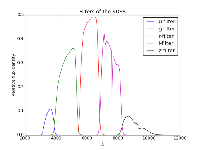
Formally, a k correction is a correction to an astronomical object’s magnitude (or equivalently, its flux) that allows a measurement of a quantity of light from an object at redshift z to be converted to an equivalent measurement in the rest frame of the object. The k corrections are also required if a comparison has to be made between observations made of objects in different bands. As an example of bands, Fig. 1 shows the filter curves that are used in the Sloan Digital Sky Survey (SDSS).
The expansion of the universe allows astronomers to convert recession velocities to radial distances. It also means that objects observed at different redshifts are sampled by any instruments at different rest-frame wavelengths. To see how this happens, recall the redshift wavelength relation:
where
and
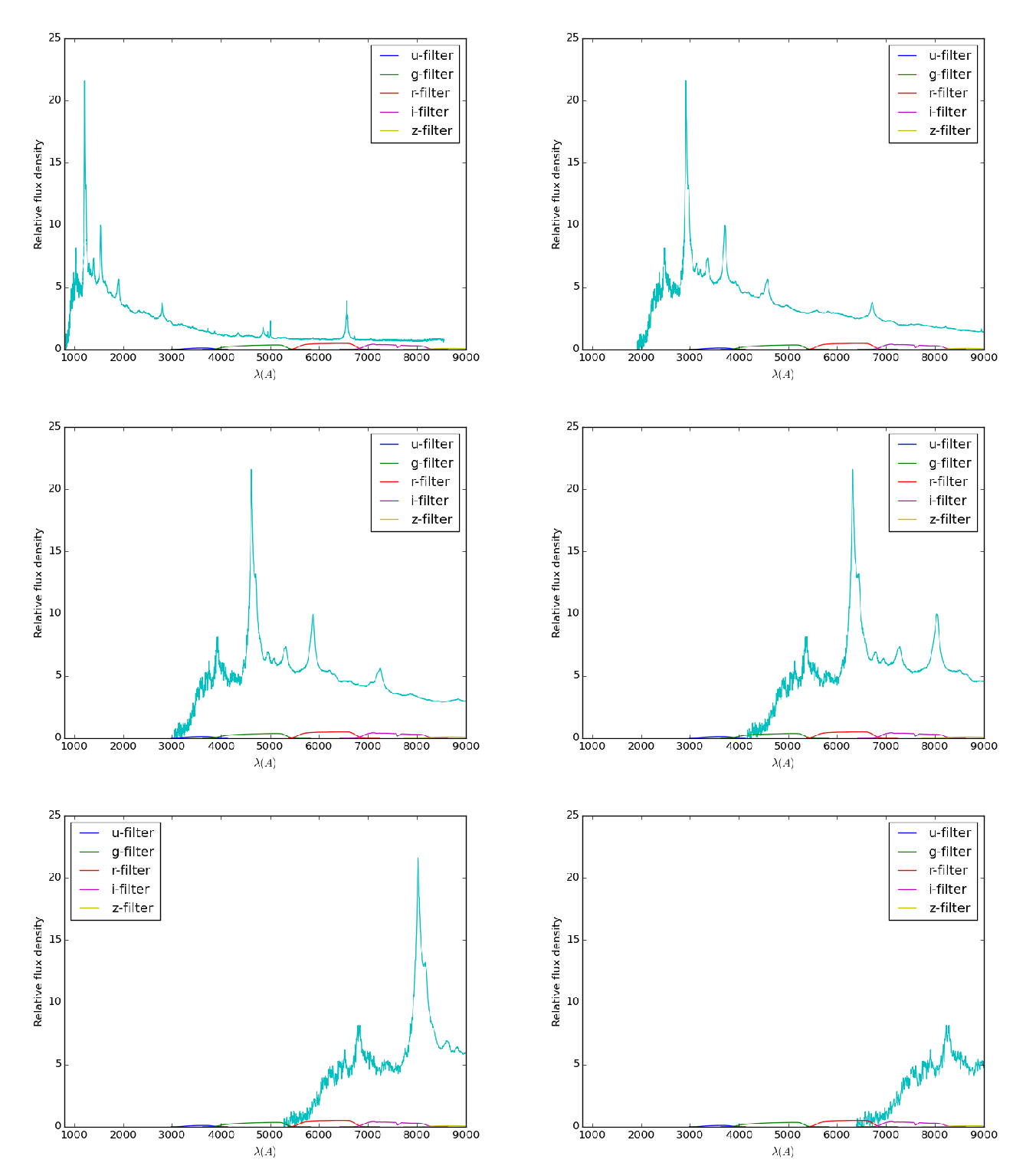
As a result, for optical observations, the measured flux of the objects corresponds to optical luminosity of nearby, or low redshift objects, whereas for higher redshift objects, it may correspond to the UV luminosity. This shift in spectra is illustrated in the animation shown below. The spectrum shown in the figure is the composite quasar spectrum, generated by Vanden Berk, et. al. The animation starts out with the spectrum as seen in the rest frame, and then displays the spectrum at consequently higher redshifts, with redshift separation of 0.05 between each spectrum.
As is clearly seen, with an increase in redshift, the spectrum shifts towards higher and higher wavelengths. As it moves towards higher wavelengths, the spectrum, with its distinct shape, moves through the various SDSS filters as well. Thus, when comparing objects at different redshifts, it is necessary to account for the shift in the spectrum, as well as scaling of the observed flux or magnitude for that object.
The Math
The simplest definition of the k correction is observed when we are talking about converting apparent magnitude to absolute magnitudes and vice versa. Mathematically, thus, it amounts to, when converting from band R to Q:
where
But eq. 2 does not actually define the k correction for us. A little bit of manipulation of eq. 2 will give us the appropriate expression for the k correction. To see how this comes about, lets first consider the equation:
This equation gives the relationship between the flux, S, and the luminosity of the object, L. This equation also serves as a definition for the luminosity distance . One important point regarding this equation is that the flux and luminosity are both bolometric, i.e. integrated over all the frequencies (instead of just confined to one passband/filter as we have discussed earlier). Due to redshift, the measured spectral flux
is related to the luminosity
, where the rest frame frequency
is related to observed frequency
by
:
Rewriting this equation in a slightly different form,
Notice that the term outside the parenthesis is the same as eq. 3, while the factor inside corrects for the spectral shift. This factor inside the parentheses is called the K-correction. But what exactly is ?
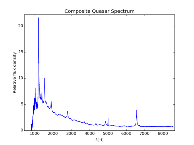
is the luminosity that is expected from the standard, composite spectrum. Thus, we need to have some information on hand about the spectrum of the object under consideration to determine the k correction. In the animation above, the spectrum shown is the composite quasar spectrum, which is used to calculate the k corrections for quasars at various redshifts. Here it is again, in case you didn’t get a good look at it while it was moving:
From this analysis, we see that we need some idea of the spectrum of the object that we wish to calculate the k correction for. However, it does not end there. So far, we have been considering only bolometric quantities (flux and luminosity). Practically, it is very difficult to measure bolometric quantities due to a variety of problems. Instead, the normal practice is to measure the flux in one or more bands, and then try to infer the properties of the object by combining the information from these various bands. This is the reason that SDSS has implemented 5 bands u, g, r, i, z, as shown in fig. 1.
Thus, the above arguments have to be redone for band-limited fluxes and magnitudes. Instead of rehashing the same argument, lets directly manipulate eq. 2. As a result, we can generalize the argument for comparisons between different filters. The complete derivation is given in this paper. Instead going through the rigorous derivation here, I will just quote the final result:
This equation is the most general definition of k correction. In this equation, the two different filters involved are denoted by R and Q. We might consider that we have observed the object in the band R, i.e. we have its apparent magnitude , and wish to know its absolute magnitude
in band Q, which is the rest frame band. In the above equation,
represents the spectral density of flux for the zero-magnitude, or “standard” source for whichever magnitude system that is in use (for example, for Vega-relative magnitudes, the the zero-magnitude is Vega). Meanwhile,
is the response for that particular filter, which is R. It is thus the probability that a photon of frequency
will be counted, over the entire range of that bandpass filter R. The same is true for the variables related to the filter Q. Thus, in addition to knowledge of the spectrum of the object, we also need to have knowledge of the filters and their response curves for the calculation of k corrections.
In conclusion, the k correction is used for comparison of objects at different redshifts. To compute redshifts, we need knowledge about the spectrum of the object of interest, along with information about the filter curves of the instrument used for making the observations. The main application of k corrections is in the study of quasars and galaxies. Both of these objects have now been detected at obscenely high redshifts, and thus, to compare them with their low redshift counterparts, a k correction is of vital importance.
To summarize in one line:
“The K-correction is the great leveler for objects from different redshifts”.
References:
[1] Wikipedia
[2] David Hogg, et. al. “The K correction”
[3] Peter Schneider, “Extragalactic Astronomy and Cosmology”, Springer


